This post is a text summary from Chetan Surpur’s slides:

Overview

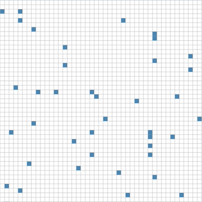
SDR is distributed and sparse, which means each bit has semantic meaning and few bits are on, more are off.

CLA is an algorithm that describes the operation of a single layer of cortical neurons. The pattern can either be spatial or temporal. Each column represents some meaning, and each cell represents the same meaning to the column but in different context (this is the key of learning high-order sequences). Learning occurs by forming and un-forming connections between neurons (cells).

Spatial Pooler

Spatial pooler maps a non-sparse representation of bits to SDR, and unions similar inputs.

Input: a vector of bits, can be the output of an encoder, or the cells in a previous layer.

Output: activation of columns.

Each cell in a column behaves identically, and the whole column is connected to inputs. Each column is mapped to a subset of input bits. More bits on, more likely the column becomes activated. The receptive field and percentage threshold of connections are controlled by potentialRadius and potentialPct. potentialPct helps adjacent columns learn to represent different inputs.

Permanence represents the potential for a connection to be formed between column and input. Minimum “connect” threshold: synPermConnected There are several ways to initialize the permanence of a cell: Gaussian, Random, etc.

To force the output to be sparse, local inhibition is used to columns within a inhibition radius. The radius is dynamic with the growth and death of connections. It’s estimated with the average range of inputs that each column is connected to, and the average number of columns each input is connected to.

Compute

1. For each column, compute an “overlap score” that represents how many input bits are “actively connected” to the column.
2. Boost if needed.
3. Check inhibition: for each column, look at the neighboring columns within inhibition radius
4. Keep the top N columns by overlap score

5. N is chosen to achieve a desired sparsity(localAreaDensity,numActiveColumnsPerInhArea)

   1 2 3 4 5 6 7 8 9 10 11 12 13 14 15 16 17 18 19 20 21 22 23 24 25 26 27 28 29 30

   def _inhibitColumns(self, overlaps): """ Performs inhibition. This method calculates the necessary values needed to actually perform inhibition and then delegates the task of picking the active columns to helper functions. Parameters: ---------------------------- :param overlaps: an array containing the overlap score for each column. The overlap score for a column is defined as the number of synapses in a "connected state" (connected synapses) that are connected to input bits which are turned on. """ # determine how many columns should be selected in the inhibition phase. # This can be specified by either setting the 'numActiveColumnsPerInhArea' # parameter or the 'localAreaDensity' parameter when initializing the class if (self._localAreaDensity > 0): density = self._localAreaDensity else: inhibitionArea = ((2*self._inhibitionRadius + 1) ** self._columnDimensions.size) inhibitionArea = min(self._numColumns, inhibitionArea) density = float(self._numActiveColumnsPerInhArea) / inhibitionArea density = min(density, 0.5) if self._globalInhibition or \ self._inhibitionRadius > max(self._columnDimensions): return self._inhibitColumnsGlobal(overlaps, density) else: return self._inhibitColumnsLocal(overlaps, density)

6. Output of SP

Learning(optional): Hebbian learning: strengthen connections to active input, and weaken connections to inactive input. And any column that becomes so weakly connected to its potential inputs that it can never become active in the future has all its connections strengthened (to keep it from dying)

Boost(optional): Strengthen connections of columns who don’t have enough overlap with their inputs (relevant parameters: minOverlapDutyCycles, synPermBelowStimulusInc). Get ready to boost in the next cycle those columns that aren’t active enough (relevant parameter: minActiveDutyCycles)

Finally, update inhibition radius.

Temporal Pooler

Temporal pooler learns transitions of SDRs. Both SP and TP operate on the same layer of cortical neurons.

Input: state of cells from last timestep and activation of columns from the current timestep.

Output: an activation of cells within columns, representing a selection of a particular context, and a prediction of cells. Predicted columns=>next predicted SDR, predicted cells=>context

Read More

– Paper by Jeff Hawkins and Subutai Ahmad

Neuron Reliability Recognize Multiple Sparse Patterns

Former View: A neuron computes a single weighted sum of all its synapses.

Active dendrites suggest a different view of the neurons, where neurons recognize many independent unique patterns. Some paper s show a small set of neighboring synapses acts as a pattern detector, and the thousands of synapses on a cell’s dendrites act as a set of independent pattern detectors.

Using sparse encoding / sub-sampling, 8-20 synapses is possible for robust recognition.

Sources of Synaptic Input to Cortical Neurons

1. Proximal synapses define the classic receptive field of a cell.
2. Basal synapses learn transition in sequences. They recognize patterns of cell activity that precede the neuron firing. (Also local inhibition)
3. Apical synapses invoke a top-down expectation. Depolarization caused by the apical dendrites is used to establish a top-down expectation (prediction).

Learning Rule

Summary: 1. learning occurs by growing and removing synapses from a pool of “potential” synapses. 2. Hebbian learning and synaptic changes occur at the level of the dendritic segment, not the entire neuron.

A threshold is used to represent the establishment of a synapse.

1

weight_of_synapse = 1 if permanence > threshold else 0

Using a scalar permanence value enables on-line learning in the presence of noise.

The activation strength of any one neuron or synapse is not very important.

Network Capacity and Generalization

Though the model is called “sequence memory”, it is actually a memory of transitions. There is no representation or concept of the length of sequences or of the number of stored sequences. The network only learns transitions between inputs.

Read More

OK, so I successfully downloaded the data from behindthenames.com. I had to resume the web crawler a couple of times when it got shut down by the web host because the web crawler is kind of DDOS attacker to the website.

There are several tricks to avoid being shut down, such as using an IP proxy, or send request to the website pretending you are using a web browser:

1

headers = {'User-Agent': 'Mozilla/5.0 (Macintosh; Intel Mac OS X 10_10_1) AppleWebKit/537.36 (KHTML, like Gecko) Chrome/39.0.2171.95 Safari/537.36'}

However, since there’re only several megabytes data to grab, I wouldn’t add these tricks to my code.

Each URL maps to a name, and each name maps to its corresponding list of name variants. Is there a better way to organize the data? The URLs do not contain any useful information to my project, so I just removed them. Another issue I have to consider is that the URLs may not point to an English name. A reversed mapping can help get rid of non-English names.

The process is:

1. Use an URL counter and store the list of name as well as name variants.

2. Reverse mapping: for each name in the lists, generate a list of URL counters.

3. Union every list mapped from the URLs in the list at step 2.

Then, for each name, there’s a set of its English variants.

1
2
3
4
5
6
7
8
9
10
11
12
13
14
15
16
17
18
19
20
21
22
23
24
25
26
27
28
29
30
31

import csv
variants = {}
for i in range(1,69):
    d = {}
    with open('lookup/'+str(i)+'.csv', 'r') as f:
        reader = csv.reader(f)
        k = 0
        for i in reader:
            d[k] = i[1:]
            k += 1
    names = {}
    for i in d.keys():
        for j in d[i]:
            if j not in names:
                names[j] = set([i])
            else:
                names[j].add(i)
    print len(names)
    for n in names:
        variants[n] = set([])
        for j in names[n]:
            variants[n] |= set(d[j])
        variants[n].remove(n)
with open('lookup.csv', 'wb') as f:
    writer = csv.writer(f)
    for v in sorted(variants.keys()):
        writer.writerow([v.upper()]+sorted(list(variants[v])))

Sample output:

1
2
3
4
5
6
7
8
9
10
11
12
13
14
15
16
17
18

'AZIZ,Aziz
'AZRI'EL,Azrael,Azriel
'EDNAH
'EFRAYIM,Efraim,Ephraim,Evron,Jevrem
'EL'AZAR,Elazar,Eleazar,Lazar,Lazare,Lazaros,Lazarus,Lazzaro
'ELI'EZER,Eliezer
'ELIFALET,'Elifelet,Eliphalet,Eliphelet
'ELIFELET,'Elifalet,Eliphalet,Eliphelet
'ESAW,Esau
'ESTER,'Ashtoret,Ashtoreth,Astaroth,Astarte,Esfir,Essi,Essie,Esta,Estee,Ester,Estera,Esteri,Esther,Esthiru,Eszter,Eszti,Hester,Hettie,Ishtar
'EZRA',Esdras,Ezra,Ezras
'IRA',Ira
'ISMAT
'ITTAY,Itai,Ithai,Ittai
'IYYOV,Ayyub,Iob,Iyov,Job,Joby
'IZEVEL
'OFRAH,Ofra,Ophrah
'ORPAH,Oprah,Orpah,Orpha

There are about 15k names, but the output csv file only takes 5.7MB space, much smaller than I had expcted.

Read More

Recently I’m working on a project, and as part of the project, I need to get data of English name variations. Asking for the internet is always the first choice. Thank Mike Campbell, I found a website www.behindthename.com/ with a huge data set of Human’s names (I mean, more than names in English are there).

Then I decided to write a web crawler to replicate a local version of the data set.

Packages

Just some standard packages for reading web pages and writing csv files.

1
2

from bs4 import BeautifulSoup
import urllib2, csv

Find out what to grab

First I browsed the website carefully.

There’s a full list of names on https://www.behindthename.com/names. For each name, all its variants can be found at www.behindthename.com/name/XXX/related.

My plan is to get the URL for each name, and then go to its ralated page, and parse its variants and save them in a list.

Get a list of URLs

1
2
3
4
5
6
7
8
9
10
11
12
13
14
15

names = []
for k in range(1, 69):
    url = 'https://www.behindthename.com/names/'+str(k)
    a,b = [],[]
    content = urllib2.urlopen(url).read()
    soup = BeautifulSoup(content, 'lxml')
    for i in soup.findAll("div", { "class" : "browsename b0" }):
        a += [i.find('a')['href'].split('/')[-1]]
    for i in soup.findAll("div", { "class" : "browsename b1" }):
        b += [i.find('a')['href'].split('/')[-1]]
    name = ['']*(len(a)+len(b))
    for i in range(len(name)):
        name[i] = a[i/2] if i%2==0 else b[(i-1)/2]
    names += name

Get list of name variants

Since I only care about English names, so I simply ignore names that cannot be encoded in ASCII.

1
2
3
4
5
6
7
8
9
10
11
12
13
14
15
16

d = {}
for n in names:
    url='https://www.behindthename.com/name/'+n+'/related'
    content = urllib2.urlopen(url).read()
    soup = BeautifulSoup(content,'lxml')
    rows = soup.findAll('a',{'class':'ngl'})
    d[n] = []
    for i in rows:
        try:
            i.string.decode('ascii')
            d[n] += [i.string.encode('ascii')]
        except UnicodeEncodeError:
            pass
    d[n] = sorted(list(set(d[n])))

It takes a while (1 hour maybe) to grab the data. #### Write CSV output

1
2
3
4

with open('lookup.csv', 'wb') as f:
    w = csv.writer(f)
    for i in d.keys():
        w.writerow([i]+d[i])

Next, I’ll do some work on efficiently accessing the data set.

Read More

Motivation:

1. We cannot directly observe the state \(x_k\in X\) of a dynamical system.

2. Measurements/observations are completely determined by system states: \(\phi: X\to \mathbb{R}\).

3. Can we reconstruct the system based on observation \(Y=(y_0, y_1, ...)=(\phi(x_0),\phi(x_1),...)\)?

Taken’s Theorem

Let \(M\) be a compact manifold of dimension \(m\). For pairs \((\phi ,y)\), with \(\phi\in Diff^2(M), y\in C^2(M,\mathbb{R})\), it is a generic (open and dense) property that the map \[ \Phi_{(\phi ,y)} : M \to \mathbb{R}^{2m+1} \]

defined by

\[ \Phi_{\phi ,y}(x) = (y(x), y(\phi(x)),...,y(\phi^{2m}(x))) \]

is an embedding.

A Demo of Takens’ Therorem

When applying Takens’ Theorem to a Lorentz system:

Blue: The original Lorentz system Green: The shadow manifold on \(X\) Orange: The shadow manifold on \(Y\) Red: The shadow manifold on \(Z\)

Code:

1
2
3
4
5
6
7
8
9
10
11
12
13
14
15
16
17
18
19
20
21
22
23
24
25
26
27
28
29
30

import numpy as np
import matplotlib.pyplot as plt
from scipy.integrate import odeint
from mpl_toolkits.mplot3d import Axes3D
rho = 28.0
sigma = 10.0
beta = 8.0 / 3.0
def f(state, t):
  x, y, z = state  # unpack the state vector
  return sigma * (y - x), x * (rho - z) - y, x * y - beta * z  # derivatives
state0 = [1.0, 1.0, 1.0]
t = np.arange(0.0, 40.0, 0.01)
tau = 5
states = odeint(f, state0, t)
fig = plt.figure()
ax = fig.gca(projection='3d')
ax.plot(states[:,0], states[:,1], states[:,2])
#plt.show()
for i in range(3):
  a = states[:,i][:-2*tau]
  b = states[:,i][tau:-tau]
  c = states[:,i][2*tau:]
  ax.plot(a,b,c)
plt.show()

Read More

Written on June 18, 2014

1.The Universe

According to Issac Newton’s theory, all the objects in the universe move regularly, and the perfect universe has neither start point nor end point. Unfortunately, this worldview contradicts with many facts people have observed. In thermodynamics, it is widely accepted and probably the truth that the universe is an isolated system so that all the spontaneous activities in the universe tend to increase the entropy, and the universe will reach thermodynamic equilibrium and end up with heat death. The dissipative structures do not violate this worldview although they could stay steadily in high-energy state but only for a while (lifetime).

2.Dissipative structure

A dissipative structure is an open system far from thermodynamic equilibrium, but keeps itself in a steady state by exchanging energy and matter with the environment. The living organisms are typical examples of dissipative structure, e.g., the distribution of temperature in the human body only has tiny fluctuations although it’s far from equilibrium. The nervous system is also a dissipative structure on the basis of body.

These structures are well organized because of they have the power of self-assembly, which decreases uncertainty among a system. In other words, self-assembly can reduce entropy. An example is that the chemistry methods are much harder than biological methods in producing macro-molecular proteins. The living organisms have special tricks to avoid internal randomness.

3.Life

Life is a dynamic process. One of the most basic features of life is self-organization (in fact, the living organisms do not have to be able to reproduce). Self-organization consumes matter, energy and keeps the operation of living organisms controllable. In the view of statistical physics, self-organization follows the migration from the most probable state to less likely states. So the entropy in the living organisms is far from maximum. In the book of “GAIA – A New Look at Life on Earth”, James Lovelock pointed out that the entropy reduction must be a general characteristic of life.

If this is true, life can possibly exist without an entity because the entropy doesn’t rely on matter exchange.

4.Entropy

This is a state variable and except for thermodynamics, it is usually defined by some probabilities. When I read the paper “Causal entropic force” again, I found difficulty in explaining intelligence only by the rule of entropy maximization. In competitive sports, players try to establish dominance so that the game will be more relax to play (fault-tolerant); in social activities, people try to make more friends. All these behaviors increase the amount of future choices (entropy). But the problem is people do not always succeed in making the most proper choice. Maybe sometimes problems are beyond the brain capacity and maybe the brain doesn’t care about the probabilities at all. This leads to the discussion of deterministic and non-deterministic.

5.Deterministic vs. non-deterministic

Except for quantum movement, I believe that uncertainty comes from the loss of information. For example, in tossing a coin, if the initial force and all the other necessary information are provided, the result of a toss should be certain. Even if only the initial acceleration is known, there should be a bias on the 0.5/0.5 probability. Another example, we can easily measure the probabilities of waiting for a traffic light by experiment, and of course the probabilities of green light coming within 1 second, and within 1 minute are different as long as the traffic light works properly. But such probabilities make no sense in predicting how long a person has to wait, which becomes deterministic if the traffic light has a countdown timer.

Non-deterministic is different from unpredictable. One is about the present and the other is about the future. A continuous time function is deterministic, but not necessarily predictable.

If we characterize a dynamical system like human brain with only state variables (e.g. Markov process) rather than process variables, the information loss would inevitably bring uncertainty. As far as my understanding, the electric charges and the synapses in a healthy human brain work in a continuous manner. On the whole, human brain works continuously all its life. This is pretty much like a manifold in topological space. If the brain knows well about its work history, there should be no internal uncertainty. The only possible uncertainty comes from the input at present. The process of giving the corresponding output is with this uncertainty but once the output is given, everything is deterministic.

Read More

1. Classifying a Set of Vectors

Let \(X\) be a set of SDRs, and for any two SDRs \(x,y\) in \(X\), \[ match(x,y)=false, \text{if} x\neq y \] Then we can tell an SDR \(z\) belongs to \(X\) if \[ \exists x\in X, match(x,z) = true \] The idea behind set \(X\) is similar with nearest neighbour algorithm on the basis of some orthogonal vectors.

2. Union

Union is used to store a set of \(M\) vectors.

\(x_1 = 00100001\)

\(x_2 = 10001000\)

\(x_3 = 10000001\)

\(x_4 = 00101000\)

\(X = x_1 OR x_2 OR x_3 OR x_4 = 10101001\)

So that a fixed-size SDR vector can store a dynamic set of elements.

3. SDRs and HTM

HTM is a detailed computational theory of the neocortex.

Read More

The Chinese room is a famous thought experiment, proposed by John Searle in 1980, which refutes the statement of “Strong AI”:

The appropriately programmed computer with the right inputs and outputs would thereby have a mind in exactly the same sense human beings have minds.

Suppose English is the only language you understand, and you are sitting in a closed room with sufficient library of books that help you do English-Chinese translation and Chinese-English translation. Your task is to interact with a Chinese speaker outside room. The question is: If the Chinese speaker feels like she’s talking with another Chinese speaker in ths task, do you literally understand Chinese?

Chinese Room and Turing Test

You don’t need knowledge of Chinese language to simulate that you understand Chinese. Machines neither.

The task itself can be seen as a Turing test, and the design is similar to Von Neumann architecture. However, the Chinese room tries to testify the existence of “consciousness” or “understanding”, which is a little irrelevant to the statement of Turing. Passing Turing test doesn’t mean a machine has any level of consciousness.

Strong AI vs. Weak AI

Most AI researchers don’t really care about the strong AI research, at least before the mind and consciousness of human can be explained by physiologists.

There is not any formal statement of what is “real intelligence” yet. Deep neural networks have got higher accuracy than human in some pattern recognition tasks, but no one would say deep learning excedds human intelligence.

Read More

I got to know HTM a year ago when my advisor told me there were internship opportunities in Jeff Hawkins’ company Numenta. Though I didn’t apply for the intern by the end, I did learn and got some basic ideas of their main product – HTM. I really appreciate the company’s persistence towards the discovery of biology-inspired artificial intelligence, especially on today when deep learning has beat more and more opponents and somehow proved the elegance of brute force.
Sparse Distributed Representation (SDR) is one of the fundamentals of HTM system. SDR can be representad as n-dimensional binary vector, in which only a small percentage of components are 1. ## 1. Biological Evidence

Sparse coding may be a general strategy of neural systems to augment memory capacity. Sparse representation of sensory information has been observed in vision, audition, touch and olfactory systems.

To any given stimulus, only very few amount of neurons have response. And any neuron in the population can only respond to a very small subset of all kinds of stimulus.

Advantages of SDR: 1. High Efficiency (energy consumption is lower than fully active neural networks) 2. Robustness (high tolerance to noises) 3. High Capacity (the overlap of representation is highly reduced)

2. Mathematical Properties of SDRs

Some basic terminologies

w: number of 1s in an SDR (vector cardinality). \(w=||x||_1\).

Overlap: number of 1s in bitwise AND (Jeff Hawkins used ON in his paper)

1
2

Overlap(01001100, 01000101) = 2
         ↑   ↑     ↑   ↑

Matching: a boolean value that is True when Overlap exceeds some threshold \(\theta\).

Uniqueness of SDR

Given vector dimension n and “norm” w, the number of unique SDRs is simply the w-Combination of set n: \(\frac{n!}{w!(n-w)!}\).

Therefore, the probability that two random SDRs are identical is very very low. (e.g. let n=1024, and w=4, the probability is 1 out of 45 billion.)

Overlap Sets

An overlap set is defined as the set of SDRs that excatly b bits overlap with SDR x, given n and w.

The size of the overlap set is the product of the number of subsets of x with b bits on, and the number of other patterns containing n-w bits, of which w-b bits are on.

\[ overlap(x,y)=x\cdot y \]

Inexact matching and subsampling

Inexact matching and subsampling are similar in finding partial matching between SDRs. There’s tradeoff between tolerance of errors (robustness) and the amount of false positives.

A false positive SDR y satisfies \(overlap(x,y)\geq\theta\).

Inexact matching decreases the right side: The lower the threshold is, the easier for a random SDR y to satisfy the inequation.

Subsampling increases the left side: the smaller the overlap set is, the easier for a random SDR y to satisfy the inequation.

Read More